Grp2_HA_Ensemble_Models

                                                                                                                               

6/8/2022                                                

Ensemble Models

June 08, 2021

 

VISHWAKARMA INSTITUTE of TECHNOLOGY

Group Members:

(04) Harsha Mamdyal, (06) Vaishnavi Mane, (07) Vedant Mane, (08) Ishan Mankar, (09) Yash Marle, (10) Pratham Matal

Guide: Prof. Deepali Joshi

 

 

Ensemble Models

In our life, at the time of making an essential decision like applying for a university program, subscribing a job contract, we tend to seek a piece of advice. We try to collect as more information as possible and reach out to multiple experts. Since similar opinions could impact our future, we trust more the decision that has been taken through similar process. Machine literacy prognostications follow a analogous geste. Models process given inputs and produce an outgrowth. The outgrowth is a prediction grounded on what pattern the models have seen during the training.

One model isn't enough in numerous cases, and this composition sheds light on this spot. When and why do we need multiple models? How to train those models? What kind of diversity those models give. So, let us right jump on the subject, but with a quick overview.

Overview

Ensemble models is a machine learning approach to combine multiple other models in the prediction process. Those models are referred to as base estimators. It is a solution to overcome the following technical challenges of building a single estimator:

High variance: The model is very sensitive to the provided inputs to the learned features.

Low accuracy: One model or one algorithm to fit the entire training data might not be good enough to meet expectations.

Features noise and bias: The model relies heavily on one or a few features while making a prediction.

Ensemble Algorithm

A single algorithm may not make the perfect prediction for a given dataset. Machine learning algorithms have their limitations and producing a model with high accuracy is challenging. If we build and combine multiple models, the overall accuracy could get boosted. The combination can be implemented by aggregating the output from each model with two objectives: reducing the model error and maintaining its generalization. The way to implement such aggregation can be achieved using some techniques. Some textbooks refer to such architecture as meta-algorithms.

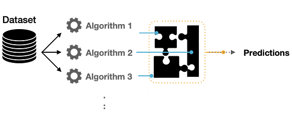
Figure 1: Diversifying the model predictions using multiple algorithms.

Ensemble Learning

Building ensemble models is not only focused on the variance of the algorithm used. For case, we could make multiple C45 models where each model is learning a specific pattern specialized in prognosticating one aspect. Those models are called weak learners that can be used to gain a meta- model. In this architecture of ensemble learners, the inputs are passed to each weak learner while collecting their predictions. The combined prediction can be used to build a final ensemble model.

One important aspect to mention is those weak learners can have different ways of mapping the features with variant decision boundaries.

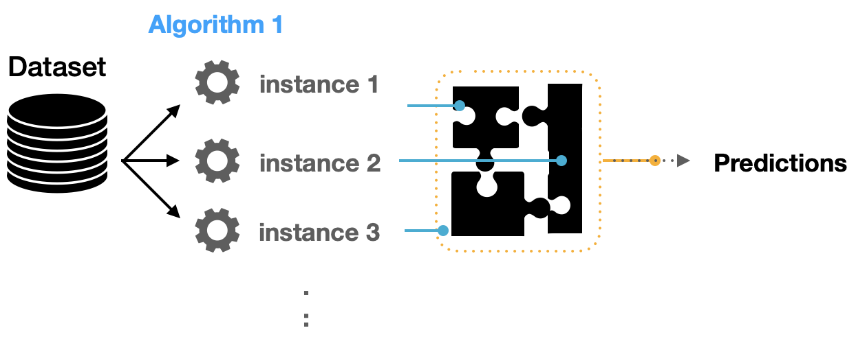
Figure 2: Aggregated predictions using multiple weak learners of the same algorithm.

Ensemble Techniques

Bagging

The idea of bagging is grounded on making the training data available to an iterative process of learning. Each model learns the error produced by the former model using a slightly different subset of the training dataset. Bagging reduces variance and minimizes overfitting. One illustration of such a fashion is the Random Forest algorithm.

1.     Bootstrapping: Bagging is grounded on a bootstrapping slice fashion. Bootstrapping creates multiple sets of the original training data with relief. relief enables the duplication of sample cases in a set. Each subset has the same equal size and can be used to train models in parallel.

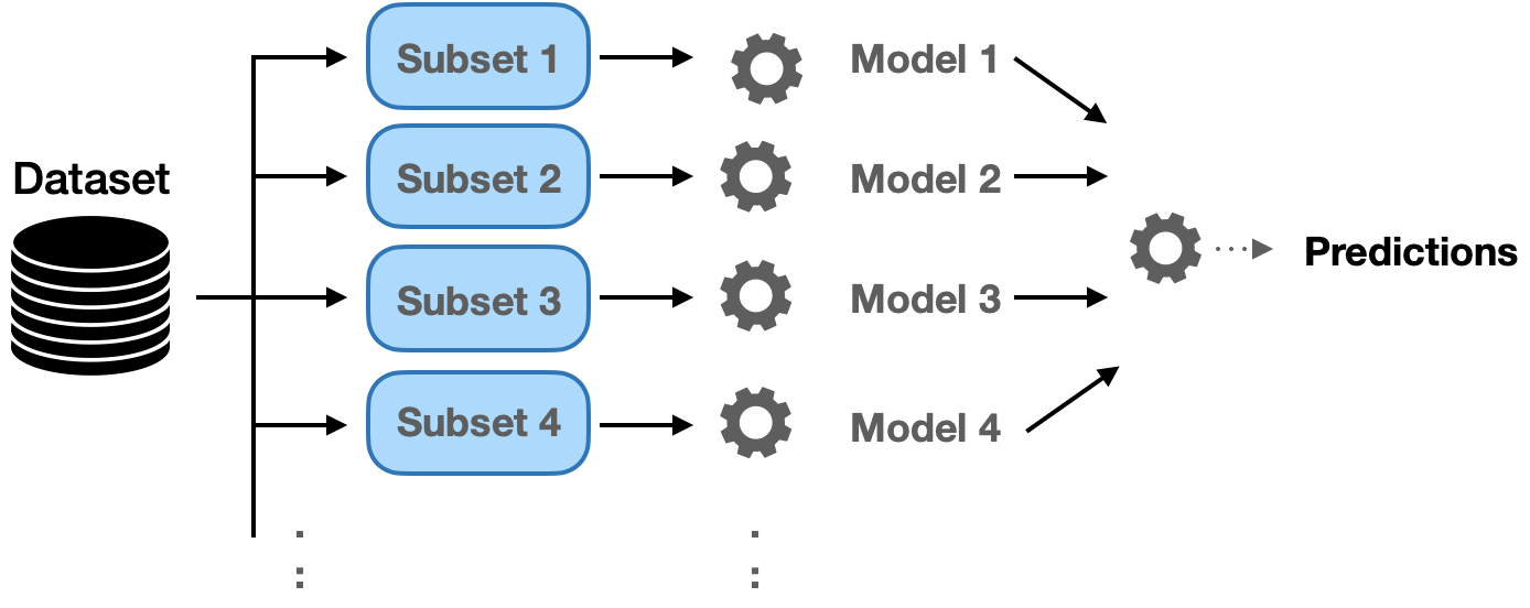
Figure 3: Bagging technique to make final predictions by combining predictions from multiple models.

2.     Random Forest: Uses subset of training samples as well as subset of features to make multiple split trees. Multiple decision trees are erected to fit each training set. The distribution of samples/ features is generally enforced in a arbitrary mode.

3.     Extra-Trees Ensemble: This is another ensemble fashion where the prognostications are combined from numerous decision trees. analogous to Random Forest, it combines a large number of decision trees. still, theExtra-trees use the whole sample while choosing the splits aimlessly.

Boosting

1.     Adaptive Boosting( AdaBoost): This is an ensemble of algorithms, where we make models on the top of several weak learners. As we mentioned before, those learners are called weak because they're generally simple with limited vaticination capabilities. The adaption capability of AdaBoost made this fashion one of the foremost successful double classifiers. successional decision trees were the core of similar rigidity where each tree is conforming its weights grounded on previous knowledge of rigor. Hence, we perform the training in such a fashion in successional rather than resemblant process. In this fashion, the process of training and measuring the error in estimates can be repeated for a given number of replication or when the error rate isn't changing significantly.

 

 

Figure 4: The sequential learning of AdaBoost producing stronger learned model.

2.     Gradient Boosting: Gradient boosting algorithms are great techniques that have high predictive performance. Xgboost, LightGBM, and CatBoost are popular boosting algorithms that can be used for regression and classification problems. Their popularity has significantly increased after their proven ability to win some Kaggle competitions.

Stacking

We've seen before that the combining models can be enforced using an aggregating system( for illustration, advancing for bracket or normal for retrogression models). mounding is analogous to boosting models; they produce further robust predictors. mounding is a process of learning how to produce such a stronger model from all weak learners ’ predictions.

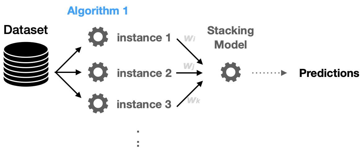
Figure 5: Stacking technique for making final prediction in an ensemble architecture.

Please note that what is being learned here (as features) is the prediction from each model.

Blending

veritably analogous to the mounding approach, except the final model is learning the confirmation and testing dataset along with prognostications. Hence, the features used is extended to include the confirmation set.

Classification Problems

Since classification is simply a categorization process. However, we need to decide shall we make a singlemulti-label classifier? or shall we make multiple double classifiers? If we decided to make a number of double classifiers, we need to interpret each model vaticination, If we've multiple markers. For case, if we want to fete four objects, each model tells if the input data is a member of that order. Hence, each model provides a probability of class. also, we can make a final ensemble model combining those classifiers.

Regression Problems

In the former function, we determine the best fitting membership using the resulted probability. In regression problems, we aren't dealing with yes or no questions. We need to find the best predicted numerical values. We can average the collected predictions.

Aggregating Predictions

When we ensemble multiple algorithms to adapt the prediction process to combine multiple models, we need an aggregating method. Three main ways can be used:

1.     Max Voting: The final prediction in this technique is made based on majority voting for classification problems.

2.     Averaging: Typically used for regression problems where predictions are averaged. The probability can be used as well, for instance, in averaging the final classification.

3.     Weighted Average: Sometimes, we need to give weights to some models/algorithms when producing the final predictions.

 

Example

We will use the following example to illustrate how to build an ensemble model. The Titanic dataset is used in this example, where we try to predict the survival of the Titanic using different techniques. A Sample of the dataset and the target column distribution to the passengers’ age are shown in Figure 6 and Figure 7.

 

Figure 6: A sample of the Titanic dataset showing that consist of twelve columns.

Figure 7: The distribution of Age column to the target.

The Titanic dataset is one of the classification problems that need extensive feature engineering. Figure 8 shows the strong correlation between some features such as Parch (parents and children) with the Family Size. We will try to focus only on the model building and how the ensemble model can be applied to this use case.

Figure 8: Correlation matrix plot of the features. dataset columns.

We will use different algorithms and techniques; therefore, we will create a model object to increase code reusability.

# Model Class to be used for different ML algorithms

class ClassifierModel(object):

    def __init__(self, clf, params=None):

        self.clf = clf(**params)def train(self, x_train, y_train):

        self.clf.fit(x_train, y_train)

    

    def fit(self,x,y):

        return self.clf.fit(x,y)

    

    def feature_importances(self,x,y):

        return self.clf.fit(x,y).feature_importances_

    

    def predict(self, x):

        return self.clf.predict(x)def trainModel(model, x_train, y_train, x_test, n_folds, seed):

    cv = KFold(n_splits= n_folds, random_state=seed)

    scores = cross_val_score(model.clf, x_train, y_train, scoring='accuracy', cv=cv, n_jobs=-1)

    return scores

 

Random Forest Classifier

# Random Forest parameters
rf_params = {
'n_estimators': 400,
'max_depth': 5,
'min_samples_leaf': 3,
'max_features' : 'sqrt',
}
rfc_model = ClassifierModel(clf=RandomForestClassifier, params=rf_params)
rfc_scores = trainModel(rfc_model,x_train, y_train, x_test, 5, 0)
rfc_scores

Extra Trees Classifier

# Extra Trees Parameters
et_params = {
'n_jobs': -1,
'n_estimators':400,
'max_depth': 5,
'min_samples_leaf': 2,
}
etc_model = ClassifierModel(clf=ExtraTreesClassifier, params=et_params)
etc_scores = trainModel(etc_model,x_train, y_train, x_test, 5, 0) # Random Forest
etc_scores

 

AdaBoost Classifier

# AdaBoost parameters
ada_params = {
'n_estimators': 400,
'learning_rate' : 0.65
}
ada_model = ClassifierModel(clf=AdaBoostClassifier, params=ada_params)
ada_scores = trainModel(ada_model,x_train, y_train, x_test, 5, 0) # Random Forest
ada_scores

 

XGBoost Classifier

# Gradient Boosting parameters
gb_params = {
'n_estimators': 400,
'max_depth': 6,
}
gbc_model = ClassifierModel(clf=GradientBoostingClassifier, params=gb_params)
gbc_scores = trainModel(gbc_model,x_train, y_train, x_test, 5, 0) # Random Forest
gbc_scores

 

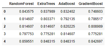
Let combine all the model cross-validation accuracy on five folds.

Now let’s build a stacking model where a new stronger model learns the predictions from all these weak learners. Our label vector used to train the previous models would remain the same. The features are the predictions collected from each classifier.

x_train = np.column_stack(( etc_train_pred, rfc_train_pred, ada_train_pred, gbc_train_pred, svc_train_pred))

Now let’s see if building XGBoost model learning only the resulted prediction would perform better. But, we will take a quick peek at the correlations between the classifiers’ predictions before that.

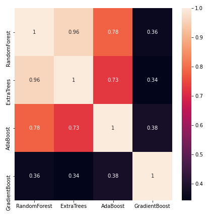
Figure 9: The Pearson correlation between the classifiers voting labels.

We will now build a model to combine the predictions from multiple contributing classifiers.

def trainStackModel(x_train, y_train, x_test, n_folds, seed):
cv = KFold(n_splits= n_folds, random_state=seed)
gbm = xgb.XGBClassifier(
n_estimators= 2000,
max_depth= 4,
min_child_weight= 2,
gamma=0.9,
subsample=0.8,
colsample_bytree=0.8,
objective= 'binary:logistic',
scale_pos_weight=1).fit(x_train, y_train)

scores = cross_val_score(gbm, x_train, y_train, scoring='accuracy', cv=cv)
return scores

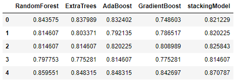
The previously created base classifiers represent Level-0 models, and the new XGBoost model represents the Level-1 model. The combination illustrates a meta-model trained on the predictions of sample data. A quick comparison between the accuracy of the new stacking model to the base classifiers are shown as follows:

 

Careful Considerations

1.     Noise, bias, and Variance: The combination of decisions from multiple models can help improve the overall performance. Hence, one of the key factors to use ensemble models is overcoming these issues: noise, bias, and variance. If the ensemble model does not give the collective experience to improve upon the accuracy in such a situation, then a careful rethinking of such employment is necessary.

2.     Simplicity and Explainability: Machine learning models, especially those put into production environments, are preferred to be simpler than complicated. The ability to explain the final model decision is empirically reduced with an ensemble.

3.     Generalizations: There are many claims that ensemble models have more ability to generalize, but other reported use cases have shown more generalization errors. Therefore, it is very likely that ensemble models with no careful training process can quickly produce high overfitting models.

4.     Inference Time: Although we might be relaxed to accept a longer time for model training, inference time is still critical. When deploying ensemble models into production, the amount of time needed to pass multiple models increases and could slow down the prediction tasks’ throughput.

Summary

Ensemble models is an excellent method for machine learning. The ensemble models have a variety of techniques for classification and regression problems. We have discovered the types of such models, how we can build a simple ensemble model, and how they boost the model accuracy.